다 5가 아니라고 판별하는 데에도 불구하고 정확도가 90이 넘게 나온다. 어떻게 이런 결과가 나오는 것일까?
숫자 5는 학습 데이터 상에서 10퍼센트 정도의 분포를 차지한다. 그래서 무조건 이것은 5가 아니라고 하면 맞을 확률이 자연스럽게 90퍼센트가 넘게 되는 것이다.
이와 비슷한 경우로 1%의 사람에게서만 발병되는 아주 희귀한 병에 대해서 진단을 할 때 관련 모델을 만들면 그 모델이 100%에 대해 그 병이 아니다라고 진단을 내리게 되면 그 진단의 Accuracy는 99%가 되나, 그 모델은 좋은 모델이라고 할 수 없는 것이다. 왜냐하면 그 병을 지닌 사람에 대해서 정확한 진단을 내릴 수 없게 되기 때문이다.
지금까지 MNIST 문제를 이진 분류해보았다. 이번엔 원래의 MNIST 분류 문제의 목적에 맞게 다중 분류를 해보도록 하자.
from sklearn.linear_model import LogisticRegression
softmax_reg = LogisticRegression(multi_class="multinomial",solver="lbfgs", C=10) # multinomial로 설정하면 multiclass에 대한 logisticregression이 가능
softmax_reg.fit(X_train, y_train)

softmax_reg.predict(X_train)[:10] # array([5, 0, 4, 1, 9, 2, 1, 3, 1, 4], dtype=uint8) # 정확히 예측하고 있다.

from sklearn.metrics import accuracy_score
y_pred = softmax_reg.predict(X_test)
accuracy_score(y_test, y_pred) # 0.9243
위의 모델을 조금 더 향상시키도록 하자.
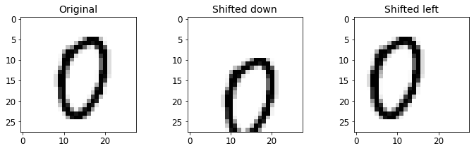
Data Augmentation
가지고 있는 학습데이터에 레이블을 유지한 채 약간의 변형을 가해 데이터를 더하여 모델을 새로 학습했을 때 조금 더 안정적인 모델을 만들어낼 수 있을 것이다.
from scipy.ndimage.interpolation import shift

# 오른쪽이나 아래로 이미지를 조금씩 shift시키는 함수
def shift_image(image, dx, dy):
    image = image.reshape((28, 28))
    shifted_image = shift(image, [dy, dx], cval=0, mode="constant")
    return shifted_image.reshape([-1])

image = X_train[1000]
shifted_image_down = shift_image(image, 0, 5) # 아래쪽으로 이동
shifted_image_left = shift_image(image, -5, 0) # 왼쪽으로 이동

plt.figure(figsize=(12,3))
plt.subplot(131)
plt.title("Original", fontsize=14)
plt.imshow(image.reshape(28, 28), interpolation="nearest", cmap="Greys")
plt.subplot(132)
plt.title("Shifted down", fontsize=14)
plt.imshow(shifted_image_down.reshape(28, 28), interpolation="nearest", cmap="Greys")
plt.subplot(133)
plt.title("Shifted left", fontsize=14)
plt.imshow(shifted_image_left.reshape(28, 28), interpolation="nearest", cmap="Greys")
plt.show()
X_train_augmented = [image for image in X_train]
y_train_augmented = [label for label in y_train]

# 레이블을 유지한 채 shift한 데이터를 추가하는 작업
for dx, dy in ((1, 0), (-1, 0), (0, 1), (0, -1)):
    for image, label in zip(X_train, y_train):
        X_train_augmented.append(shift_image(image, dx, dy))
        y_train_augmented.append(label)

X_train_augmented = np.array(X_train_augmented)
y_train_augmented = np.array(y_train_augmented)

X_train_augmented.shape # (300000, 784) # 원래의 데이터보다 5배만큼 늘어났다.

# 같은 레이블의 데이터가 연속으로 있으면 모델을 학습하는 데 있어서 좋지 않은 영향을 끼칠 것이다. 그래서 데이터를 섞어주는 작업을 하자.
shuffle_idx = np.random.permutation(len(X_train_augmented))
X_train_augmented = X_train_augmented[shuffle_idx]
y_train_augmented = y_train_augmented[shuffle_idx]

# 모델 학습
softmax_reg_augmented = LogisticRegression(multi_class="multinomial",solver="lbfgs", C=10)
softmax_reg_augmented.fit(X_train_augmented, y_train_augmented)

y_pred = softmax_reg_augmented.predict(X_test)
accuracy_score(y_test, y_pred) # 0.9279 # data augmentation을 진행하기 전보다 0.002정도 오른 것을 확인할 수 있다.
# 0.002면 작은 수치일 수도 있으나, 이미 잘 나온 모델에서 조금이라도 정확도를 올렸다는 것은 굉장히 유의미한 일이다.
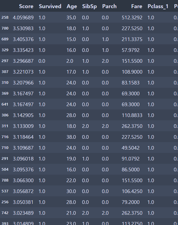
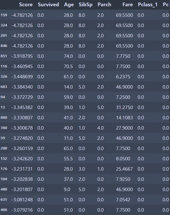
Titanic 데이터셋에 대해 분류하기
import numpy as np
import pandas as pd

train_data = pd.read_csv("titanic.csv")
속성들
Survived: that's the target, 0 means the passenger did not survive, while 1 means he/she survived.
Pclass: passenger class.
Name,Sex,Age: self-explanatory
SibSp: how many siblings & spouses of the passenger aboard the Titanic.
Parch: how many children & parents of the passenger aboard the Titanic.
Ticket: ticket id
Fare: price paid (in pounds)
Cabin: passenger's cabin number
Embarked: where the passenger embarked the Titanic
이 중 Ticket같은 경우는 고유한 번호가 될 가능성이 높은데 고유한 식별자를 feature data로 쓰면 학습을 할 때 고유한 정보를 외우는 수준까지 갈 수도 있기 때문에(이 고유한 식별자에 집중하게 될 수도 있기 때문에) 예측값이 굉장히 안 좋아질 수도 있다. 그렇기 때문에 사용하지 않는 것이 더 좋다고 볼 수 있다.